11.6. Generate 1D Phantom data
11.6.1. Goal
The goal of this tutorial is to use the Phantom generation tool for,
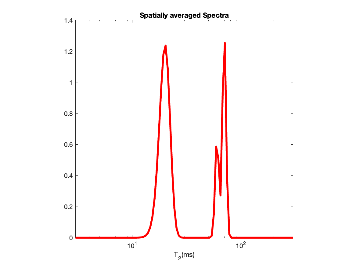
Generating DRSuite compatible (see here for format) 1D \(T_2\)-Relaxation Phantom data with a ground truth spectral peaks as shown below,
|
|
Figure 1. Ground truth spectral peaks |
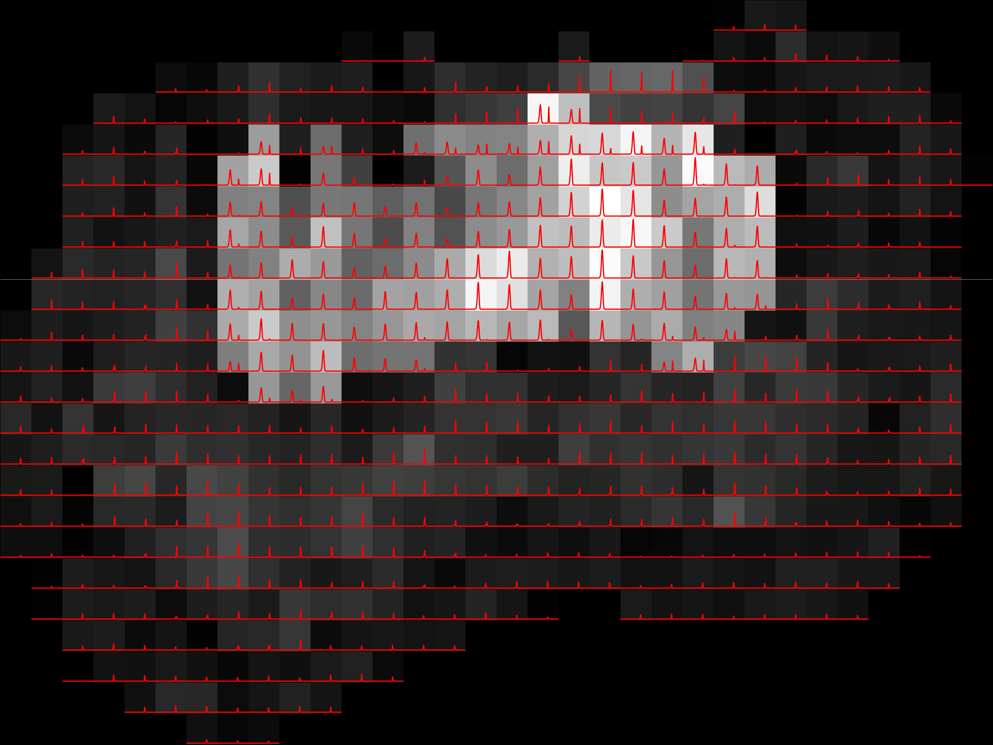
Figure 2. Spatial Distribution of the spectral peaks |
Creating two mask files, one for penalty parameter selection and another for spectral estimation.
Creating the spectrum information related file to be used in spectrum estimation.
Citation
If you use this phantom, please cite:
Kim et al., Diffusion-relaxation correlation spectroscopic imaging: A multidimensional approach for probing microstructure, 2017. DOI: 10.1002/mrm.26629
11.6.2. Relevant links
Before getting started with the software, the user is required to download the following files
acq_phantom1D.txt,Phantom1D_spect.txtfrom thislinkhere. We are providing these files as an example input to the Phantom generation tool.acq_phantom1D.txtcontains information about the T2 contrast encodings andPhantom_spect1D.txtcontains the specification for spectral sampling points.Full guide to install DRSuite software tools can be found here.
For matlab based implementation, please download the folders namely,
'utilities','solver','ini2struct'and the function'create_phantom.m'provided in the github here (add url).
11.6.3. Get started
For MATLAB based implementation, open matlab in the directory where you have unzipped the above downloaded files. Assume that directory is the ‘Documents’ folder. For Linux commandline, just open the terminal in the ‘Documents’ folder. So ideally the ‘Documents’ folder will have the following files:
/Documents/
├── acq_phantom1D.txt
├── Phantom1D_spect.txt
├── utilities (For MATLAB only)
├── solver (For MATLAB only)
├── ini2struct (For MATLAB only)
└── create_phantom.m (For MATLAB only)
Run the command below for matlab based implementations to add the folders (assuming they are on the ‘Documents’ folder), not required for Linux based implementations:
addpath("solvers","utilities","ini2struct")
Now let us look at the
acq_phantom1D.txtfile. This file contains a total of 35 contrast encodings (b-values fixed, TE value changes) and providing this as an input will generate MR data at each of these encodings. Note that the units for b and TE values are \(ms/\mu m^2\) and \(ms\) respectively. If you are willing to provide your own acquisition parameter, please use the same unit. Also, each acquisition should be in one row with b-value first then TE value seperated by comma. This file looks like below,0,10 0,20 0,30 ... 0,350
Note
The difference between 1D T2-Relaxation phantom and Diffusion relaxation Phantom generation is that for the former case, we provide fixed b-value and only TE-values change but for the latter case, both the (b,TE) value changes (as you can check from the
acq_phantom1D.txtfile mentioned in step 3 in this tutorial). Also if you want to create 1D Diffusion Phantom, provide (b,TE) combination with changing b-values and fixed TE value.The another file
Phantom1D_spect.txtgives information about the spectral parameters. The file is given below:T2_min=3; T2_max=1000; T2_spacing='log'; T2_num=300;
This file when given to the Phantom generation tool, will help generating the spectrum information file as we discussed here. This specification generates the only spectral axes points with
T2_numlogarithmically spaced points betweenT2_minandT2_max. Note that you may change the values of the variables (i.e., changeT2_min=3toT2_min=30) but the variable names should never be changed (e.g., changingT2_numtoT2_numsort2_numwill give erroneus result). All units should be in \(ms\). Also note that as we are dealing with 1D Phantom, we only specified spectral informations only corresponding toT2values and skipped the informations corresponding to diffusion coefficient (D) parameters. If you change theacq_Phantom1D.txtfile to have only b-value changing with TE fixed, you need to provide spectrum specification that informes software about diffusion coefficient,D. In this case also all units should be in \(\mu m^2/ms\). An example.txtfile is given below,D_min=0.04; D_max=4; D_spacing='log'; D_num=200;
Now run the tool to generate the 1D T2-Phantom. In the following inputs, we have set
'multislice'/-multisliceto 0 to produce one slice in the final MR data. We could have also skipped using this'multislice'/-multisliceargument because by default the Phantom generation tool generates single slice.create_phantom.sh -acqfile 'acq_phantom1D.txt' -spectfile 'Phantom1D_spect.txt' -multislice 0 -outfolder 'Phantom1D'
create_phantom('acqfile','acq_phantom1D.txt','spectfile','Phantom1D_spect.txt','outfolder','Phantom1D','multislice',0)
For more details about the inputs to the above function see here.
11.6.4. Outputs
This will generate the following folder with four files:
/Documents/Phantom1D/
├── Phantom_data.mat
├── Phantom_spectrum_info.mat
├── Phantom_mask.mat
└── Phantom_mask_beta_calc.mat
Phantom_data.mat — spatial MR data (see imgfile)
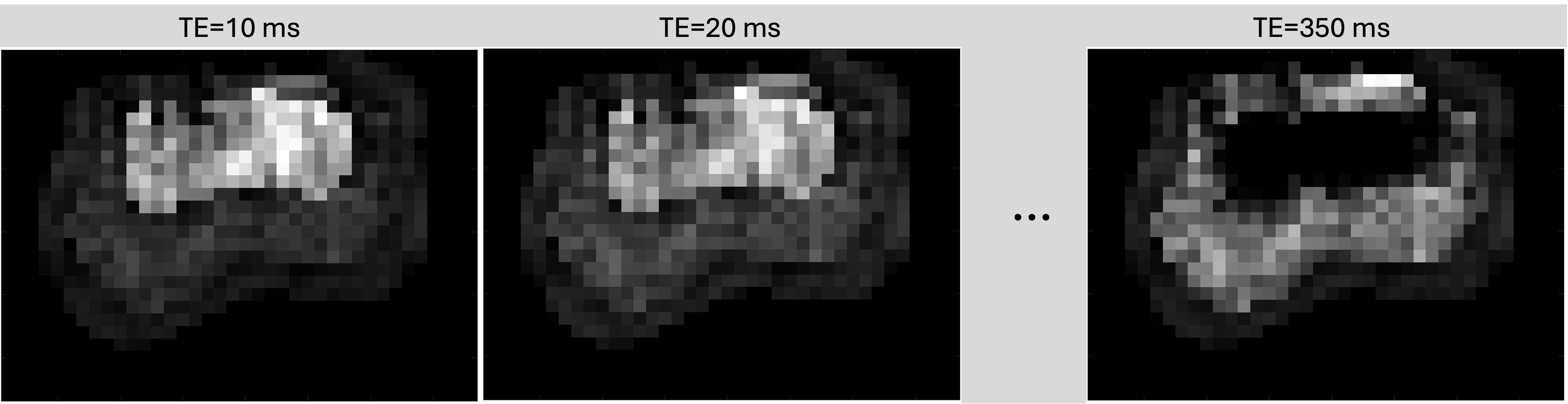
data: 4-D double, size[35, 28, 38]; 2D MR Magnitude image for 35 (b,TE) combinations (although b value is fixed).resolution:[Δx, Δy, Δz]in mm (In this example we have hardcoded the resolution to:[1, 1, 1])spatial_dim:[28, 38](number of voxels per axis)transform: 4×4 affine (voxel → world, Identity matrix)
The MR data looks as below (three encodings),
Phantom_spectrum_info.mat — spectrum metadata + dictionary (see spectrumInfofile)
K: double matrix, size[35, 300], the dictionary file generated for mapping the spectrum amplitudes to MR data of 35 contrast encodingsaxes: 1×1 struct with fields:sample(1×M_i vector),name(char),unit(char),spacing('log'or'linear')axis 1 (relaxation): name
'T_2', unit ‘\(ms\)’, 300 samples, spacing'log'.
spectral_dim:300, storing the spectral dimension for axis 1.
Phantom_mask.mat — binary spatial mask (see spatialMaskfile)
im_mask: logical, size[28, 38](1 → voxels inside Phantom ROI, 0 → voxels outside Phantom ROI)
Phantom_mask_beta_calc.mat — binary mask patches for ADMM/LADMM penalty parameter selection
im_mask: logical, size[28, 38](Contains two 3x3 mask patches for each slice)