11.4. Estimating Spectrum from Generated 2D Phantom data

The most crucial tool in this software is to estimate the spectrum from the multidimensional MR data. For an unknown spectrum \(\boldsymbol{f}_i\) for \(i\)-th voxel, we solve following nonegatively constrained optimisation problem with spatial smoothness regulariser,

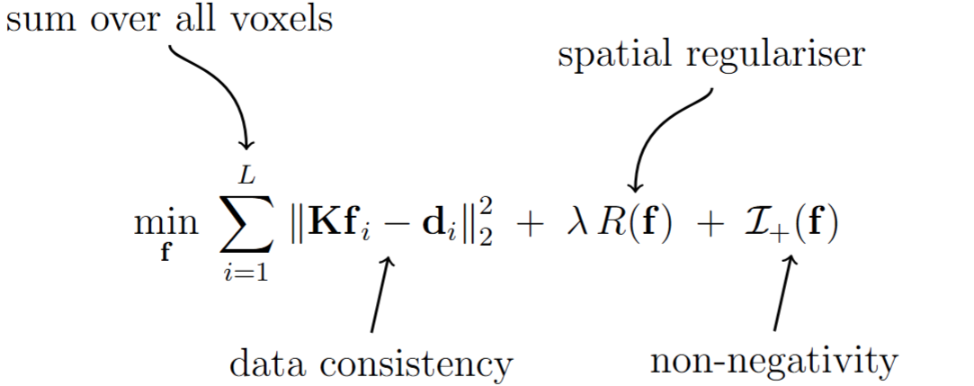
where \(\boldsymbol{\mathrm{d}}_i\) is the vectorised multidimensional MR data acquired from the voxel \(i\) and \(\boldsymbol{\mathrm{f}}\) is the vector formed by concatenating the unknown spectra from all \(L\) voxels. \(\boldsymbol{\mathrm{K}}\) is the dictionary matrix that maps the spectral amplitude to the MR data. We have shown here how to create the dictionary tensor. We just flatten the spectral dimension of the dictionary tensor to get the above mentioned matrix form. The novelty of this method is the use of the spatial smoothness regulariser term along with more general non-negativity constraint. This spatial smoothness regulariser minimises the the difference between the neighboring voxels’ spectra. This paper elaborately explains the concecpt behind the regulariser. The smoothness is controlled by the regularization parameter \(\lambda\). If you choose lambda too large, you may get solutions that look over-smoothed. If you choose lambda too small, you may get solutions that are too noisy to be useful. This is an engineering trade-off, and it is up to the user to identify what they like. In the tutorial below, we show this behavior with examples. This spatially regularized reconstruction is often hundreds of times better than unregularized reconstruction from an estimation theoretic point of view (cite), although is computationally slower. We provide two algorithms for regularized reconstruction: LADMM (which is often the fastest cite), ADMM (which is generally slower but is still provided for reference cite), and the conventional unregularized NNLS solution (which is very fast but frequently produces worse results). These can be chosen by appropriately stting parameters in the configuration file.

11.4.1. Goal

This tutorial will guide you to estimate the spectrum from the 2D phantom data generated in the last tutorial. Specifically we will be,

Creating the configuration file (as discussed here) to specify algorithm parameters for spectrum estimation.
Choosing optimal penalty parameter for ADMM/LADMM algorithm
Finally estimating spectrum using relevant files.

Citation

If you use ADMM algorithm for your spectral estimation, please cite:

Kim et al., Diffusion-relaxation correlation spectroscopic imaging: A multidimensional approach for probing microstructure, 2017. DOI: 10.1002/mrm.26629

Liu et al., An Efficient Algorithm for Spatial-Spectral Partial Volume Compartment Mapping With Applications to Multicomponent Diffusion and Relaxation MRI,2025. DOI: 10.1109/TCI.2025.3609974

If you use LADMM algorithm for your spectral estimation, please cite:

Liu et al., An Efficient Algorithm for Spatial-Spectral Partial Volume Compartment Mapping With Applications to Multicomponent Diffusion and Relaxation MRI,2025. DOI: 10.1109/TCI.2025.3609974

11.4.2. Get started

Before going to the process of estimating spectra, lets check if we have the folder with the following files (we will be working in the Documents directory):

/Documents/Phantom2D/
├── Phantom_data.mat
├── Phantom2d_data_noisy.mat (downloaded)
├── Phantom_spectrum_info.mat
├── Phantom_mask.mat
└── Phantom_mask_beta_calc.mat

Once we have these files, we have to create configfile to provide details of the algorithm. We have created the following .ini file using the text editor to use LADMM algorithm and saved it in the ‘Documents’ folder with file name 'Phantom2D_ladmm.ini'.
```
dc_comp = 1
lambda = 0.001

[solver]
name = 'LADMM'
num_iter = 4000
beta = 1.0
save_inter = 100
tol = 5e-5
check_tol = 500

[low_rank]
flag = 1
rank = 20
```
This file specifies the parameters of the spectrum estimation tool:

Top-level (global)
- dc_comp: Assigning to 1 we are enabling the estimation algorithm to get rid of any constant offset present in the data. If the data does not seem to have a constant offset value, we can assign ‘dc_comp’ value to 0. Only required for ADMM or LADMM algorithm.
- lambda parameter is the value of spatial regulariser. Higher value of this parameter will result in smoother spectrum. Only required for 'ADMM' or 'LADMM' algorithm. 'NNLS' does not support usage of the spatial regulariser.
[solver]
- name: Solver to run, For this tutorial we chose to use 'LADMM' algorithm. Change the name to choose from other two available algorithms - 'ADMM' , 'NNLS'. 'NNLS' solves the first optimization problem mentioned above, whereas 'ADMM' or 'LADMM' solves the second optimzation problem.
- num_iter: Maximum iterations before stopping (hard cap). Set to 2000 here. If the tolerance criteria as mentioned below is not met, the algorithm will stop after 2000 iteration. Higher number of iteration will make sure the final spectra is a converged solution.
- beta: LADMM penalty parameter, chosen 1.0 arbitrarily. Follow the next step to fine tune this value for faster convergence.
- save_inter: Save intermediate outputs 100 iterations in this case. Output types vary depending on the function used.
- tol: Convergence tolerance on the stopping metric. If the tolerance value of 5e-5 is achieved before num_iter the spectrum estimation process will stop.
- check_tol: Check the stopping criterion after 500 iteration for skipping the initial transient behavior of cost function. If the tol value is reached before check_tol iterations, the algorithm won’t stop, because the tolerance value is checked after check_tol iterations.
[low_rank]
- flag: Enable/disable low-rank approximation of the matrix, K (1 = on, 0 = off).
- rank: Target rank for the matrix K. Lower the rank, faster the LADMM algorithm. The user should choose the rank by looking at the distribution of the singular values of the tensor, K.
See more details about each entry of this configuration file here.
Although we have provided a beta value in the config file, we are not sure if that is going to give us fastest convergence for the above dataset. So now we will create another text file containing beta values to compare convergence speed. Open a text editor and save the file with name ‘betafile_phantom2d.txt’ in ‘Documents’ folder. Note that the variable name should always be ‘beta_vals’ in the text file.
```
beta_vals= [0.05 0.5 1 5];
```
Now the we can run the tool that will calculate the convergence speed for the above beta values. Note that our Phantom generation code generates two spatial masks, one for the whole MR volume and another for the penalty parameter selection. We use the second spatial mask named 'Phantom2D/Phantom_mask_beta_calc.mat' in this case. You can also create your own patches of masks following the mask file format. We recommend having multiple 3x3 patches for each slice and choose the region such that you include spatial region having most partial voluming.
SH
plot_beta_sweep.sh -imgfile 'Phantom2D/Phantom_data.mat' -betafile 'betafile_phantom2d.txt' -spect_infofile 'Phantom2D/Phantom_spectrm_info.mat' -configfile 'Phantom2D_ladmm.ini' -spatmaskfile 'Phantom2D/Phantom_mask_beta_calc.mat' -outprefix 'Phantom2D/Phantom2D_data_ladmm_spect' -file_types 'png'
MATLAB
plot_beta_sweep('imgfile','Phantom2D/Phantom_data.mat','betafile','betafile_phantom2d.txt', 'spect_infofile','Phantom2D/Phantom_spectrm_info.mat','configfile','Phantom2D_ladmm.ini','spatmaskfile','Phantom2D/Phantom_mask_beta_calc.mat','outprefix','Phantom2D/Phantom2D_data_ladmm_spect','file_types','png')
This will save the image ‘Phantom2D/Phantom2D_data_ladmm_spect_costVSiter_multi_beta.png’ as shown below. As you can see that the convergence rate is the fastest for beta = 0.5. So now we change the beta value from 1.0 to 0.5 in the configfile, 'Phantom2D_ladmm.ini'. You can also fine tune the beta value by repeating step 3 with updated multiple beta_vals closely spaced around 0.5.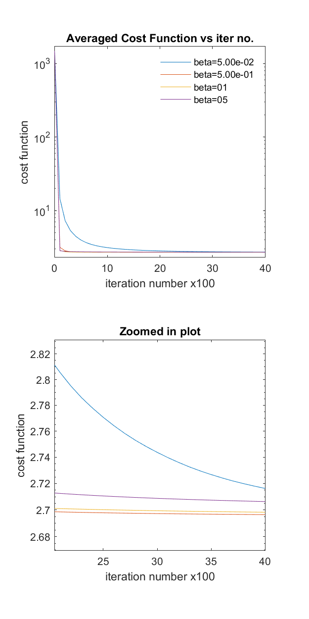

Note

This plot of cost function vs iteration number for multiple beta can give us an approximate number of maximum iterations required for achieving a converged solution. As you can see from the figure above that, for beta= 0.5, 1, and 5 the cost function is not changing much after 2000 iterations (so, converged!), whereas, the cost function still haven’t converged for beta = 0.05. So if you choose beta value of 0.05 and use num_iter value to 4000, you will not ever get a converged solution. Most of the times, these unconverged solution vary significantly from the converged solution. So its better to start with a higher value of num_iter to generate the above plot. This way we can get an idea about the maximum iteration number, approximately needed for the whole volume spectrum estimation.
Once we have all the required files set, we can run the spectral estimation solver,
SH
estimate_spectra.sh -imgfile 'Phantom2D/Phantom_data.mat' -spect_infofile 'Phantom2D/Phantom_spectrm_info.mat' -configfile 'Phantom2D_ladmm.ini' -spatmaskfile 'Phantom2D/Phantom_mask.mat' -outprefix 'Phantom2D/Phantom2D_data_ladmm_spect'
MATLAB
estimate_spectra('imgfile','Phantom2D/Phantom_data.mat', 'spect_infofile', 'Phantom2D/Phantom_spectrm_info.mat','configfile','Phantom2D_ladmm.ini','spatmaskfile','Phantom2D/Phantom_mask.mat','outprefix','Phantom2D/Phantom2D_data_ladmm_spect')
This will store the spectrosocpic image in the file as specified by out_prefix in MATLAB v7.3 (HDF5) format and will also generate an image (named out_prefix_costVsiter_single_beta.png) storing the total cost function from all the voxels vs iteration plot for the estimated spectra. This plot is shown below,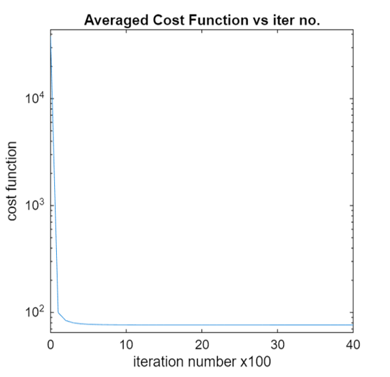

The above plot shows that the cost function is converged and the user can reliably trust the estimated spectra. If low value of num_iter or tol is used, then the cost function may not converge.

Note

You can turn off plotting the cost function vs iteration plot and potentially save some time by not calculating cost function at regular intervals, but having this figure to check if the estimated spectra is the converged solution of the optimization problem mentioned above is highly beneficial.
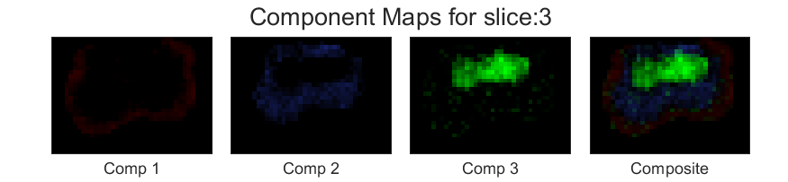
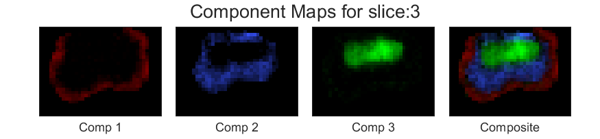
Although we have put up a seperate visualization tutorial, here we show the component maps from the spectra to qualitatively judge the effects of the spatial regulariser. As each component in the component maps is calculated by summing a spectral region from the spectra of each voxel, the component maps can directly infer the effect of the spatial regulariser (for more details follow the documentation). Below we can see the component maps corresponding to the third slice for the spatial regulariser value, \(\lambda=0.0001\),
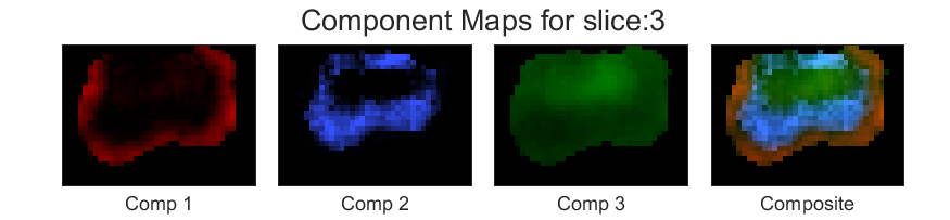
Now lets choose another \(\lambda=.01\). The component maps for the same slice looks as follows,

You can see that the component maps has smoothened a bit.

Note

Although changing \(\lambda\) alters the convergence characteristics of the optimisation problem, here we are showing the results after appropriately setting other parameters in the configuration file.

Next we are choosing bigger regularization parameter, \(\lambda=1\). The component maps are generated as follows,

As you can see, changing the value of the regularisation parameter is a trade-off between sptial resolution and noise. and among the above three different spatial regulariser, the one with \(\lambda=0.01\) achieves reasonable noise characteristics without excessive loss of spatial resolution.
Similarly you can play with other parameters in the configuation file, such as change the total number of iteration, increase the tolerance value etc to estimate the spectra.
Now let’s change the solver from 'LADMM' to 'NNLS'. Generating the configfile for this solver is very easy; We only need to create the .ini file as below,
```
[solver]
name = 'NNLS'
```
The component maps are shown below,

We can see that the only non negatively constrained optimisation for estimating the spectra is resulting in very noisy output for this Phantom data and does not contain any meaningful information.

11.4.3. Output

This command will save the estimated spectrum in the file named ‘Phantom2D/Phantom2D_data_ladmm_spect.mat’.

Phantom2D_data_ladmm_spect.mat — spectroscopic image file (see here)
- spectral_image: double matrix, size [70,70,28,38,5], the 70x70 spectrum for each of the 28x38x5 volxels in one file.
- axes: 1×5 struct with fields: type (char), sample (1×N vector), name (char), unit (char), spacing ('log' or 'linear')
  - axis 1 (diffusion): type, 'spectral', name 'D', unit ‘\(\mu m^2/ms\)’, 70 samples, spacing 'log'.
  - axis 2 (relaxation): type, 'spectral', name 'T_2', unit ‘\(ms\)’, 70 samples, spacing 'log'.
  - axis 3 : type, 'spatial', name 'x', unit ‘\(mm\)’, empty samples, spacing 'linear'.
  - axis 4 : type, 'spatial', name 'y', unit ‘\(mm\)’, empty samples, spacing 'linear'.
  - axis 5 : type, 'spatial', name 'z', unit ‘\(mm\)’, empty samples, spacing 'linear'.
- spectral_dim: [70, 70], storing the spectral dimension for axes 1 and axes 2 respectively.
- spatial_dim`: ``[28, 38, 5], storing the spatial dimension for axes 3, 4 ,5 respectively.
- transform: 4×4 affine (voxel → world, Identity matrix)
- resolution: [Δx, Δy, Δz] in mm.

Note that some variables in this file are directly transferred from the 'Phantom_spectrm_info.mat' file. In the next tutorial we will be visualising the estimated spectra.