11.5. Visualising Estimated Spectra for 2D Phantom Data

11.5.1. Goal

This tutorial will guide you through the visualising process of the estimated spectra from the 2D Phantom data as generated in this tutorial. By the end of this tutorial you will be able to

Visualise spatially resolved spectra using plotSpectIm.
Plot averaged spectra across selected spatial regions using plotAvgspect.
Create spectral mask and plot component maps using the spectral mask using plotCompMaps.
Adjust figure appearance (e.g., axis scale, colorbar, axis limits, colormap etc).
Export the resulting figures in different file formats for documentation or further analysis.

11.5.2. Relevant downloads

This tutorial requires you to download the files Phantom_spectrum_mask.mat and four_color.mat from this link. The first file contains four spectral roi’s that we have already generated and stored in this format and the second file stores the information related to the color of each components and follows the format mentioned here.

11.5.3. Get started

Before going to the visualisation, lets check if we have the following file in our working directory (for this tutorial also we are assuming we are working in the ‘Documents’ folder)

/Documents/
├── Phantom2D/Phantom2D_data_ladmm_spect.mat (Generated from spectrum estimation tool)
├── Phantom2D/Phantom_data.mat (Generated from Phantom generation tool)
├── Phantom2D/Phantom_mask.mat (Generated from Phantom generation tool)
├── Phantom_spectrum_mask.mat (downloaded)
└── four_color.mat (downloaded)

11.5.4. Plot Spectroscopic image:

We will be using the function plotspectIm.sh/plotspectIm.m to plot the spectroscopic images. The detailed documentation is given here. Spectroscopic image is the visualisation of each individual spectrum spatially located at the source voxel location and the spectrum’s back ground is the MR data intensity of that voxel. The user can choose subset of region for which spectroscopic image will be plotted, select the color of each individual spectrum, zoom into to spectrum at all the selected voxels etc using this tool. In this tutorial we will be exploring the usage of the above function.

First plot the spectroscopic image with the default setting and required inputs:
SH
plot_spect_im.sh -spect_imfile 'Phantom2D/Phantom2D_data_ladmm_spect.mat' -imgfile 'Phantom2D/Phantom_data.mat' -outprefix 'Phantom2D/Phantom2D_data_spectroscopic_Im' -spatmaskfile 'Phantom2D/Phantom_mask.mat'
MATLAB
plot_spect_im('spect_imfile','Phantom2D/Phantom2D_data_ladmm_spect.mat','imgfile','Phantom2D/Phantom_data.mat','outprefix','Phantom2D/Phantom2D_data_spectroscopic_Im','spatmaskfile', 'Phantom2D/Phantom_mask.mat')
The above program will generate the following slicewise spectroscopic images namely, ‘Phantom2D/Phantom2D_data_spectroscopic_Im_*.png’ (‘*’- denoting slice numbers) for all the voxels indexed in the whole volume mask file ‘Phantom2D/Phantom_mask.mat’ by 1’s.

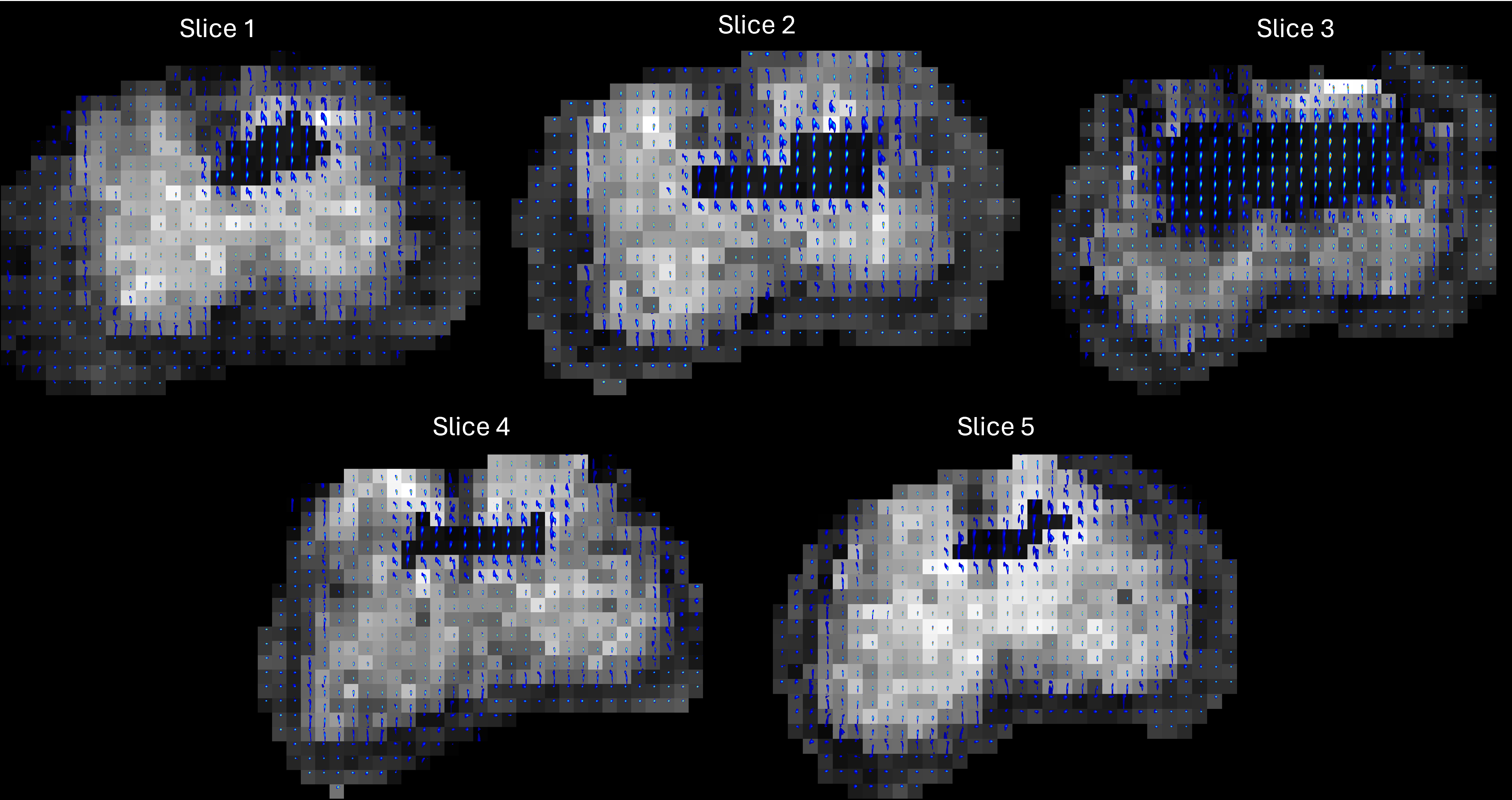
These plots are generated with the default setting in the tool. Now, let’s use the optional inputs to better explore the spectroscopic images.
We can tune the figure appearance by changing the optional inputs. Lets say we want to zoom into the region for \(0.03<D<2\) and \(10<T_2<100\). This is controlled by the named argument ax_lims. We set it to \([0.03 \; 2 \; 10 \; 100]\). Lets also change the color for each spectrum to the 'parula', plot the second contrast encoding of the multidimensional MR image as background for each slice, set background threshold to 0.25 and save them in two types of format, ‘png’ and ‘eps’. The tool is run as follows with the above inputs,
SH
plot_spect_im.sh -spect_imfile 'Phantom2D/Phantom2D_data_ladmm_spect.mat' -imgfile 'Phantom2D/Phantom_data.mat' -outprefix 'Phantom2D/Phantom2D_data_spectroscopic_Im' -spatmaskfile 'Phantom2D/Phantom_mask.mat' -ax_lims '[0.01 1.5 10 100]' -color 'parula' -enc_idx 2 -threshold 0.25 -file_types 'png' 'eps'
MATLAB
plot_spect_im('spect_imfile', 'Phantom2D/Phantom2D_data_ladmm_spect.mat', 'imgfile','Phantom2D/Phantom_data.mat', 'outprefix', 'Phantom2D/Phantom2D_data_spectroscopic_Im', 'spatmaskfile', 'Phantom2D/Phantom_mask.mat','ax_lims',[0.03 2 10 100], 'color','parula', 'enc_idx', 2, 'normalise', 1, 'threshold', 0.25, 'file_types', {'png','eps'})
Below we show the slice 3 generated from the above command.

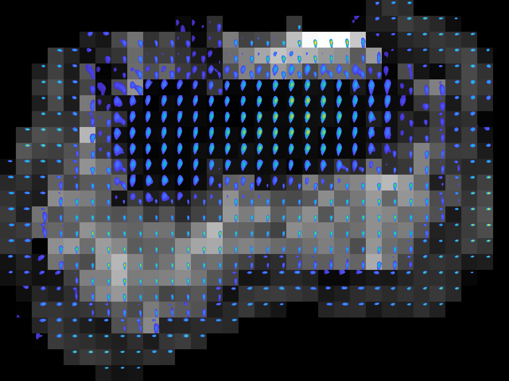
All the images above shows the voxelwise spectra and their spatial distribution which is very important to analyse the estimated spectra and underlying tissue properties.

11.5.5. Plot Average Spectra:

We will be using the function plotAvgSpectra.m/plotAvgSpectra.sh to plot the average spectra from all the voxels specified by the spatial mask. Detailed documentation is given here.

Let’s run the tool using the following command and defaults inputs:

SH

plot_avg_spectra.sh -spect_imfile 'Phantom2D/Phantom2D_data_ladmm_spect.mat' -outprefix 'Phantom2D/Phantom2D_data_ladmm_avg_spectra' -spatmaskfile 'Phantom2D/Phantom_mask.mat'

MATLAB

plot_avg_spectra('spect_imfile','Phantom2D/Phantom2D_data_ladmm_spect.mat','outprefix','Phantom2D/Phantom2D_data_ladmm_avg_spectra','spatmaskfile','Phantom2D/Phantom_mask.mat')

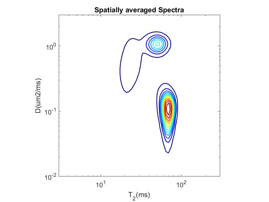
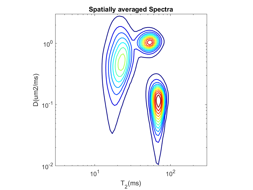
This will generate the following contour plot showing the average spectra from all the voxels indicated by 1 in the spatial maskfile ‘Phantom2D/Phantom_mask.mat’.

We can modify the spatial mask to generate average spectra from each individual slices. For a binary mask, same as the dimension of the data, we need to only set value 1 to the locations which defines the region corresponding to a particular slice and zero in all the other locations. We have provided such five .mat files, 'Phantom_mask_slice_*.mat' (‘*’->1,2,…5) for all the individual slices. Below we run the command for slice no 3 and the corresponding average spectra follows.
SH
plot_avg_spectra.sh -spect_imfile 'Phantom2D/Phantom2D_data_ladmm_spect.mat' -outprefix 'Phantom2D/Phantom2D_data_ladmm_avg_spectra' -spatmaskfile 'Phantom2D/Phantom_mask_slice_3.mat'
MATLAB
plot_avg_spectra('spect_imfile','Phantom2D/Phantom2D_data_ladmm_spect.mat','outprefix','Phantom2D/Phantom2D_data_ladmm_avg_spectra','spatmaskfile','Phantom2D/Phantom_mask_slice_3.mat')

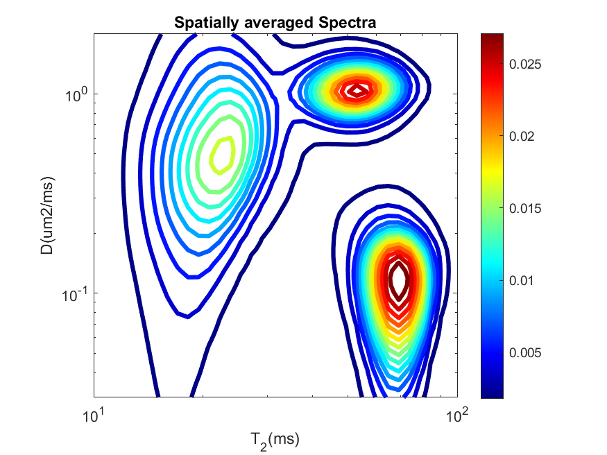
We can also change appearance of the figure by modifying the optional inputs as done before while plotting the spectroscopic image. There are few common named arguments, which work the same way as in the previous tool. These are, ax_lims, color, file_types. However, here we can also change the axes scaling (using ax_scale), number of levels in the contour plots (using nlev), line width of the contours (using linewidth) and add colorbar (using cbar) to the plot. We have applied all these arguments to revisualize of the average spectra for slice 3,

SH

plot_avg_spectra.sh -spect_imfile 'Phantom2D/Phantom2D_data_ladmm_spect.mat' -outprefix 'Phantom2D/Phantom2D_data_ladmm_avg_spectra' -spatmaskfile 'Phantom2D/Phantom_mask.mat' -ax_scale 'log' -ax_lims '[0.01 3 3 300]' -color 'jet' -nlevel 15 -linewidth 3 -cbar 1 -file_types 'png'

MATLAB

plot_avg_spectra('spect_imfile', 'Phantom2D/Phantom2D_data_ladmm_spect.mat', 'outprefix', 'Phantom2D/Phantom2D_data_ladmm_avg_spectra', 'spatmaskfile','Phantom2D/Phantom_mask.mat', 'ax_scale', 'log', 'ax_lims', [0.03 2 10 100],'color','jet','nlevel',15,'linewidth',3,'cbar',1,'file_types','png')

The average spectra now looks as follows,

11.5.6. Plot Component Maps:

One of the most crucial step to generate component maps is to create the spectral ROI (note that this is different from the spatial mask as described in the above examples). Component maps are constructed by the signal from specific spectral region. We generate the spectral ROI to define such specific spectral regions. This spectral ROI is a \(M_1 \times M_2 \times N_c\) (for 2D spectrum, where \(M_p\) is the \(p\)-th spectral dimension and \(N_c\) is the user defined total number of components) binary mask where the locations in the mask equal to 1 are the spectral regions that we are interested in.

We know that the estimated spectra signifies the amplitude of the spectra at the spectral sampling points used while creating the dictionary. The Spectral ROI indexes these spectral sampling points. If we have only single location in the spectral ROI to be one, then we will get an image showing the spatial distribution of the amplitude values corresponding to that one specific spectral sampling point. If we have multiple points for which the spectral ROI is one, then we will get an image showing the spatial distribution of the sum of the amplitudes across all of the indicated spectral sampling points. These images are called component maps. Mathematically, for a voxel location \((x,y,sl)\) the intensity of the t-th component map is calculated as follows,

\[I_t(x,y,sl)=\sum_{(i,j)\in \Lambda_t} f(i,j,x,y,sl)\]

Where \(\Lambda_t\) is the region in the 2D spectral ROI with value \(1\) and \(f(i,j,x,y,sl)\) is the 2D spectrum amplitudes for a 3D spatial volume as calculated from the spectrum estimation tool.

First let’s create the spectral ROI. As the spectral_dim has value [70 70], we need to create binary matrix of dimension 70x70 with zeros everywhere except the spectral region whose component maps we are interested to evaluate. In this tutorial we will look into the component maps corresponding to three spectral regions, so we created three binary masks as below to visualise the component maps corresponding to the spectral regions indicated by the white pixels below,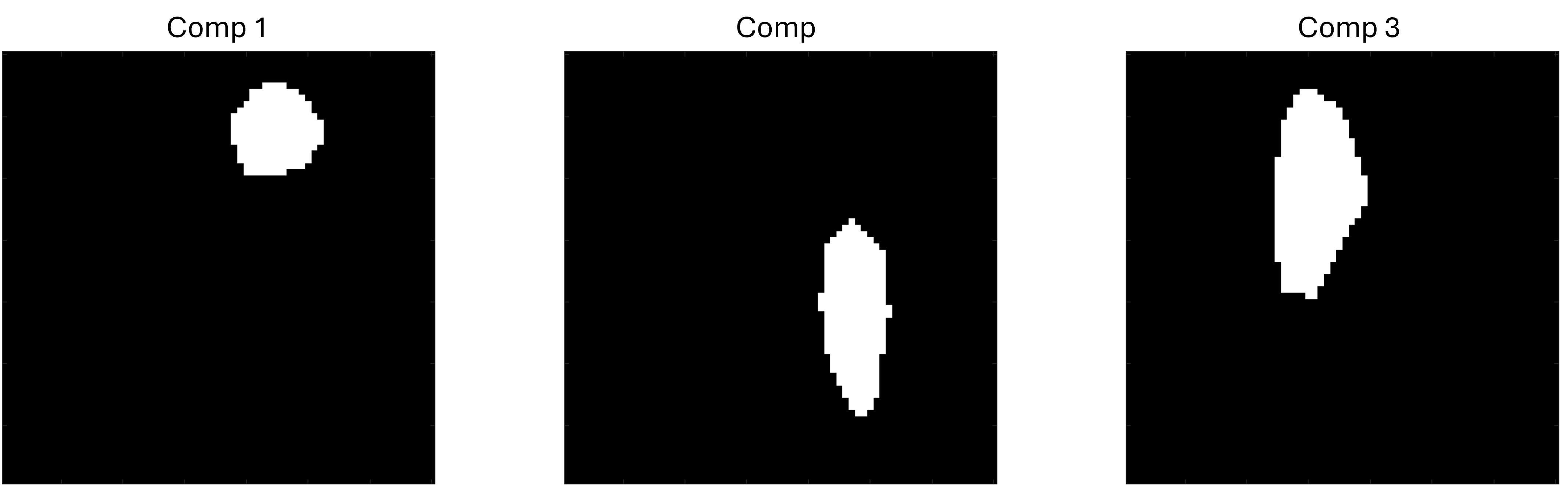
Lets name the matrices storing the above 70x70 masks as roi1, roi2, roi3``. Next we need to create the spectrum mask file with the format as given here. In this regard we need to create two variables named spec_mask and num_comp. The first variable stores all the spectral mask and the second variable stores the number of components. We have to concatenate these three 70x70 spectral masks to create spec_mask of dimension 70x70x3 and assign value 3 to the num-comp variable. Below is the MATLAB implementation to create such variable and store them to the file named ‘Phantom_spectrum_mask.mat’.
```
num_comp=3;
spec_mask=cat(3,roi1,roi2,roi3);
save('Phantom_spectrum_mask.mat',"spec_mask","num_comp",'-v7.3')
```
Note

Although we have used four components here, you can create as many as 13 components if you are using default colors while plotting the component maps. If you have more than 13 component to visualise, please create a colorfile with the format mentioned here.
Once we have the spectral mask, ‘Phantom_spectrum_mask.mat’ (either created following steps 1-2 above or by downloading the above zip file), we can use it to plot the the component maps. Detailed description is available here. We run the tool using the following required name value pairs,
SH
plot_comp_maps.sh -spect_imfile 'Phantom2D/Phantom2D_data_ladmm_spect.mat' -spectmaskfile 'Phantom_spectrum_mask.mat' -outprefix 'Phantom2D/Phantom2D_data_component_maps'
MATLAB
plot_comp_maps('spect_imfile','Phantom2D/Phantom2D_data_ladmm_spect.mat','spectmaskfile','Phantom_spectrum_mask.mat','outprefix','Phantom2D/Phantom2D_data_component_maps')
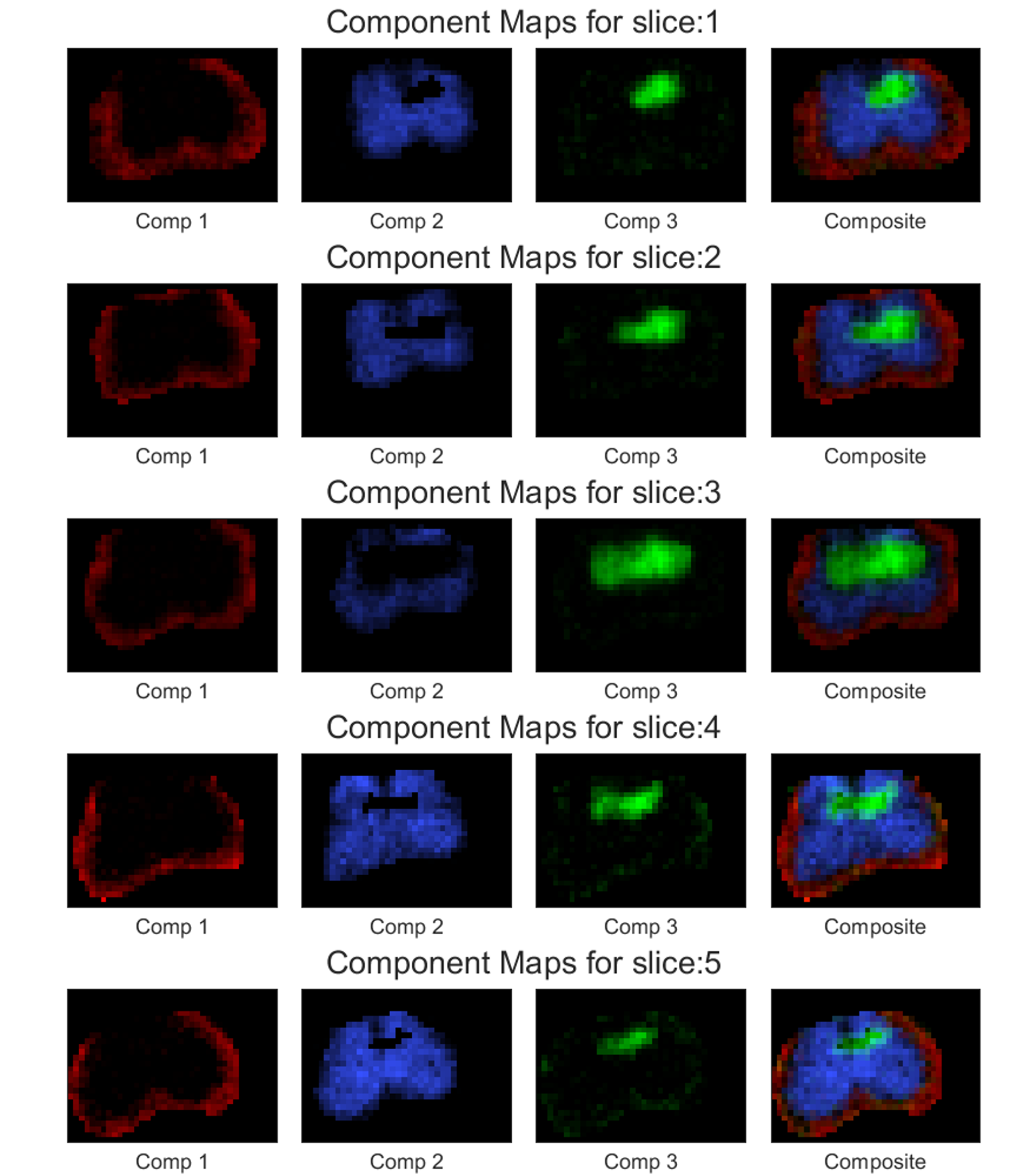
The above command will store five images named ‘Phantom2D/Phantom2D_data_component_maps_*.png’ (‘*’-> slice number) corresponding to the component maps for all the slices and a .mat file named ‘’Phantom2D/Phantom2D_data_component_maps.mat’ storing the component map data in a similar format as in mentioned here. The component maps are shown below: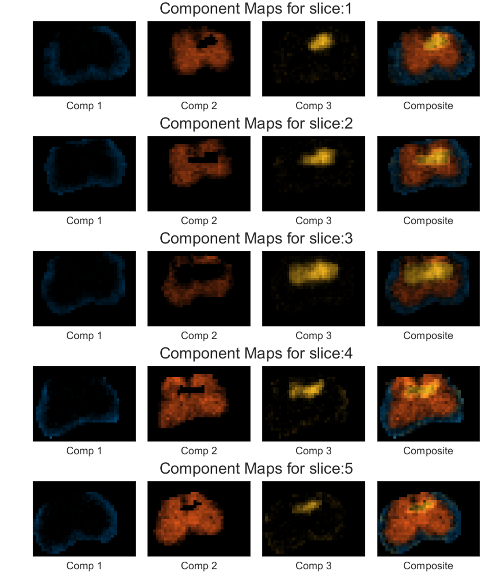
The above program generates slicewise component maps corresponding to the four spectral regions chosen with the default colors. If you want to use a custom color, you can use the colorfile, 'four_colors.mat' provided in the above downloadable zip file. This input is controlled by the named argument , color (format can be found here). As you may see from the above image that component 1 for all the slices looks darker, we can change its appearance using the argument weights. We have set it to [1 2 1 1] so that the brightness for component 2 increases, so does its intensity in the composite maps. We can also add colorbar to each of these component maps using cbar and output image file format using file_types.
SH
plot_comp_maps.sh -spect_imfile 'Phantom2D/Phantom2D_data_ladmm_spect.mat' -spectmaskfile 'Phantom_spectrum_mask.mat' -outprefix 'Phantom2D/Phantom2D_data_component_maps' -color 'four_color.mat' -weights [1 2 1 1] -cbar 1 -file_types 'png'
MATLAB
plot_comp_maps('spect_imfile','Phantom2D/Phantom2D_data_ladmm_spect.mat','spectmaskfile','Phantom_spectrum_mask.mat','outprefix','Phantom2D/Phantom2D_data_component_maps','color','four_color.mat','weights',[1 2 1 1],'cbar',1,'file_types','png')
Below is the component maps for slice 3,