11.3. Generate 2D Phantom data

11.3.1. Goal

The goal of this tutorial is to use the Phantom generation tool for,

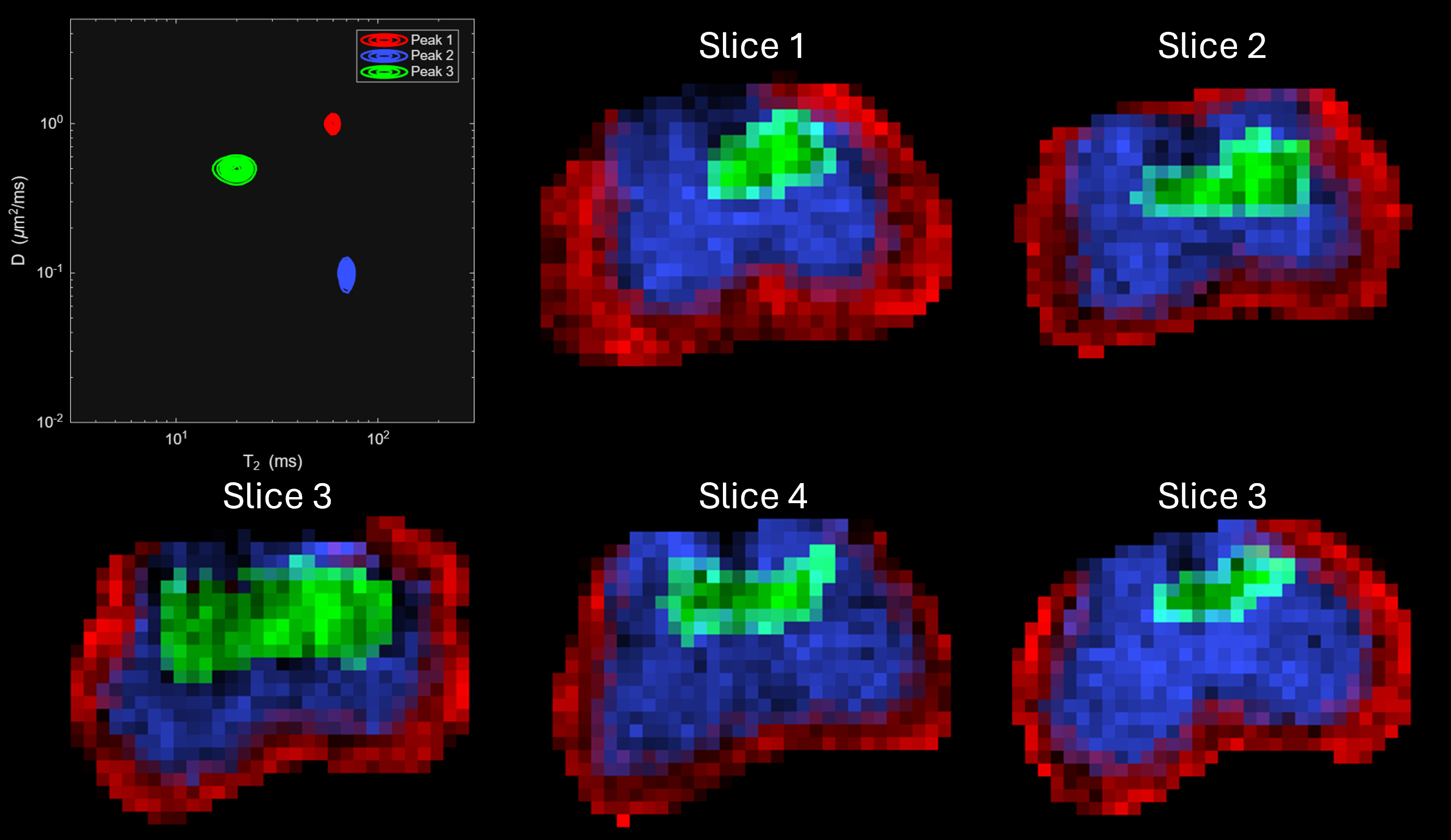
• Generating DRSuite compatible (see here for format) Diffusion-Relaxation Phantom data with ground truth spectral peaks and their slicewise spatial distribution as shown below,

• Creating two mask files, one for penalty parameter selection and another for spectral estimation.

• Creating the spectrum information related file to be used in spectrum estimation.

Citation

If you use this phantom, please cite:

Kim et al., Diffusion-relaxation correlation spectroscopic imaging: A multidimensional approach for probing microstructure, 2017. DOI: 10.1002/mrm.26629

11.3.2. Relevant links

• Before getting started with the software, the user is required to download the following files acq_phantom.txt, Phantom_spect.txt from this link here. We are providing these files as an example input to the Phantom generation tool. acq_phantom.txt contains information about the contrast encodings and Phantom_spect.txt contains the specification for spectral sampling points.

• Full guide to install DRSuite software tools can be found here.

• For matlab based implementation, please download the folders namely, 'utilities', 'solver', 'ini2struct' and the function 'create_phantom.m' provided in the github here (add url).

11.3.3. Get started

1. For MATLAB based implementation, open matlab in the directory where you have unzipped the above downloaded files. Assume that directory is the ‘Documents’ folder. For Linux commandline, just open the terminal in the ‘Documents’ folder. So ideally the ‘Documents’ folder will have the following files:

   /Documents/
   ├── acq_phantom.txt
   ├── Phantom_spect.txt
   ├── utilities (For MATLAB only)
   ├── solver (For MATLAB only)
   ├── ini2struct (For MATLAB only)
   └── create_phantom.m (For MATLAB only)
   

2. Run the command below for matlab based implementations to add the folders (assuming they are on the ‘Document’ folder), not required for Linux based implementations:

   addpath("solvers","utilities","ini2struct")
   

3. Now let us look at the acq_phantom.txt file. This file contains a total of 49 contrast encodings (b-TE combinations) and providing this as an input will generate MR data at each of these encodings. Note that the units for b and TE values are \(ms/\mu m^2\) and \(ms\) respectively. If you are willing to provide your own acquisition parameter, please use the same unit. Also, each acquisition should be in one row with b-value first then TE value seperated by comma. This file looks like below,

   0,99
   0,120
   0,160
   ...
   5,400
   

4. The another file Phantom_spect.txt gives information about the spectral parameters. The file is given below:

   D_min=0.01;
   D_max=3;
   D_spacing='log';
   D_num=70;
   T2_min=3;
   T2_max=300;
   T2_spacing='log';
   T2_num=70;
   

   This file when given to the Phantom generation tool, will help generating the spectrum information file as we discussed here. This specification generates D_num logarithmically spaced sampling points for the first axes (which is the diffusion coefficient) with the end point values being D_min and D_max. Similary, this also generates the second spectral axes points with T2_num logarithmically spaced points between T2_min and T2_max. Note that you may change the values of the variables (i.e., change D_num=70 to D_num=100) but the variable names should never be changed (e.g., changing D_num to D_nums or d_num will give erroneus result).

5. Now run the tool to generate the 2D Phantom. In the following inputs, we have set 'multislice'/-multislice to 1 to have two slices in the final MR data. you can set it to 0 to generate single slice. Also you can change the outfolder name but here we have used 'Phantom2D' to have consistency in the later tutorials.

   SH

   create_phantom.sh -acqfile 'acq_phantom.txt' -spectfile 'Phantom_spect.txt' -multislice 1 -outfolder 'Phantom2D'
   

   MATLAB

   create_phantom('acqfile','acq_phantom.txt','spectfile','Phantom_spect.txt','outfolder','Phantom2D','multislice',1)
   

   For more details about the inputs to the above function see here.

11.3.4. Outputs

This will generate the following folder with four files:

/Documents/Phantom2D/
├── Phantom_data.mat
├── Phantom_spectrum_info.mat
├── Phantom_mask.mat
└── Phantom_mask_beta_calc.mat

• Phantom_data.mat — spatial MR data (see imgfile)

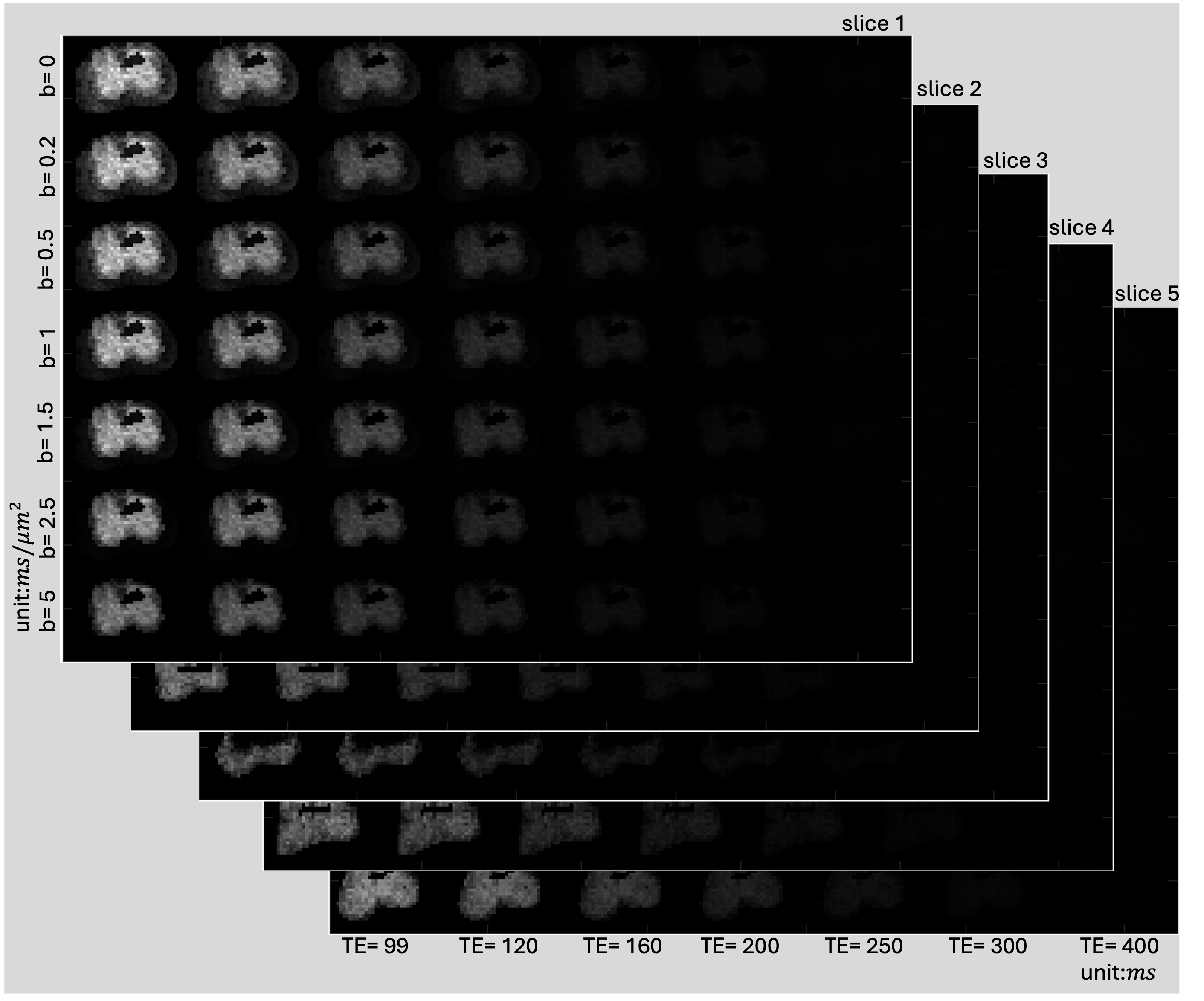
  • data: 4-D double, size [49, 28, 38, 5]; 3D MR Magnitude image for 49 (b,TE) combinations.

  • resolution: [Δx, Δy, Δz] in mm (In this example we have hardcoded the resolution to: [1, 1, 1])

  • spatial_dim: [28, 38, 5] (number of voxels per axis)

  • transform: 4×4 affine (voxel → world, Identity matrix)

  The slice wise MR data looks as below,

  

• Phantom_spectrum_info.mat — spectrum metadata + dictionary (see spectrumInfofile)

  • K: double matrix, size [49, 70, 70], the dictionary file generated for mapping the spectrum amplitudes to MR data of 49 contrast encodings

  • axes: 1×2 struct with fields: sample (1×N vector), name (char), unit (char), spacing ('log' or 'linear')

    • axis 1 (diffusion): name 'D', unit ‘\(\mu m^2/ms\)’, 70 samples, spacing 'log'.

    • axis 2 (relaxation): name 'T_2', unit ‘\(ms\)’, 70 samples, spacing 'log'.

  • spectral_dim: [70, 70], storing the spectral dimension for axis1 and axis 2 respectively.

• Phantom_mask.mat — binary spatial mask (see spatialMaskfile)

  • im_mask: logical, size [28, 38, 5] (1 → voxels inside Phantom ROI, 0 → voxels outside Phantom ROI)

• Phantom_mask_beta_calc.mat — binary mask patches for ADMM/LADMM penalty parameter selection

  • im_mask: logical, size [28, 38, 5] (Contains two 3x3 mask patches for each slice)

In the next tutrial we will estimate the spectra using thee files generated in the Phantom2D folder.