6. Spectroscopic Image Estimation
Given a set of coregistered multicontrast MRI images in imgfile format, the spectEstimation.sh tool can be used to perform spectroscopic image estimation. This tool is designed to solve the following spatially-regularized nonnegativity-constrained optimization problem
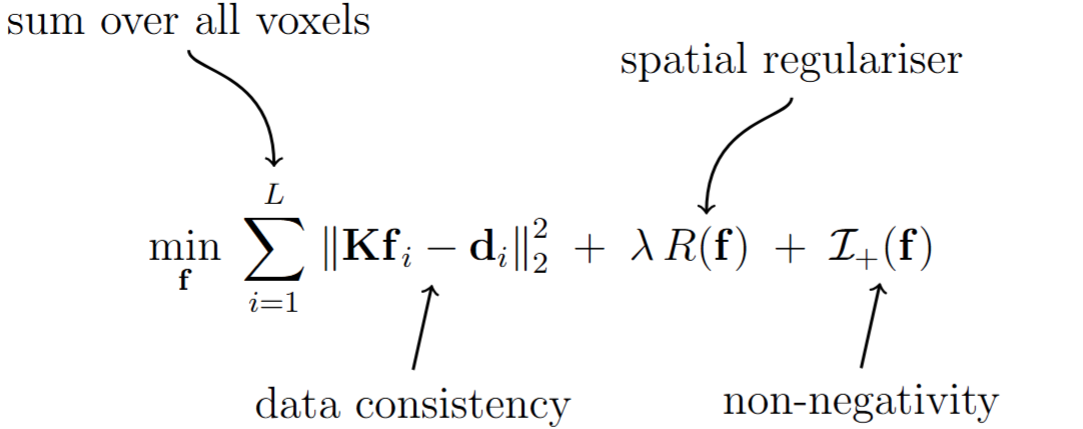
where \(\mathbf{f}_i\) is the spectrum corresponding to the \(i\)th voxel, \(\boldsymbol{\mathrm{d}}_i\) is the vector of multicontrast MR image amplitude values from \(i\)th voxel, and \(\boldsymbol{\mathrm{f}}\) is the vector formed by concatenating the unknown spectra from all \(L\) voxels. \(\boldsymbol{\mathrm{K}}\) is the dictionary matrix that describes how the image contrast is expected to vary for different tissue contrast parameters (e.g., diffusion and/or relaxation) across the different experimental settings that were used in the acquisition (e.g., \(b\)-value, TE, etc.). For example, to estimate a diffusion-relaxation spectrum \(f(D,T2)\) for a set of \(M_1\) diffusivity gridpoints \(D_1,\ldots,D_{M_1}\) and \(M_2\) relaxation gridpoints \(T2_1,\ldots T2_{M_2}\) for an acquisition with \(N_a\) images, where the \(n\)th acquisition has contrast paramters \((b_n, TE_n)\), then the matrix \(\mathbf{K}\) will be of size \(N_a \times M_1 M_2\) and could have entries of the form \(e^{-b_n D_{m_1}} e^{- TE_n/T2_{m_2}}\).
To run the solver, it is necessary to create a spect_infofile as described here, which defines the spectral grid of parameter values to be estimated as well as the corresponding dictionary matrix \(\mathbf{K}\). It is also necessary to create a configfile as described here, which defines the algorithm and algorithm parameters used by the solver. Some of the most impactful algorithm choices include:
Regularization parameter. The regularization parameter \(\lambda\) can be varied to achieve a good balance between the ill-posedness and noise sensitivity of the algorithm versus the spatial resolution of the estimated spectroscopic image. Larger \(\lambda\) is associated with better conditioning and noise suppression, at the expense of worse spatial resolution and increased blurring.
Algorithm. We provide two algorithms for regularized reconstruction:
The LADMM algorithm (which is often the fastest). This algorithm is described in the following paper, which should be cited, along with DRSuite, when using this choice:
Liu, D. Mandal, C. Liao, K. Setsompop, J. P. Haldar. An Efficient Algorithm for Spatial-Spectral Partial Volume Compartment Mapping with Applications to Multicomponent Diffusion and Relaxation MRI. IEEE Transactions on Computational Imaging 11:1283-1293, 2025. <https://doi.org/10.1109/TCI.2025.3609974>
The ADMM algorithm (the original algorithm for spatially-regularized estimation, which is generally slower than LADMM but is still provided for reference). This algorithm is described in the following papers, which should be cited, along with DRSuite, when using this choice:
Kim, E. K. Doyle, J. L. Wisnowski, J. H. Kim, J. P. Haldar. Diffusion-Relaxation Correlation Spectroscopic Imaging: A Multidimensional Approach for Probing Microstructure. Magnetic Resonance in Medicine 78:2236-2249, 2017. <https://dx.doi.org/10.1002/mrm.26629>
Kim, J. L. Wisnowski, C. T. Nguyen, J. P. Haldar. Multidimensional Correlation Spectroscopic Imaging of Exponential Decays: From Theoretical Principles to In Vivo Human Applications. NMR in Biomedicine 33:e4244, 2020. <https://doi.org/10.1002/nbm.4244>
Liu, D. Mandal, C. Liao, K. Setsompop, J. P. Haldar. An Efficient Algorithm for Spatial-Spectral Partial Volume Compartment Mapping with Applications to Multicomponent Diffusion and Relaxation MRI. IEEE Transactions on Computational Imaging 11:1283-1293, 2025. <https://doi.org/10.1109/TCI.2025.3609974>
The NNLS algorithm (which is classical and very fast, but only performs voxel-by-voxel spectrum with nonnegativity constraints and is incompatible with spatial regularization. When using this approach, \(\lambda\) must be set to zero).
Beta Both the LADMM and ADMM algorithms depend on the choice of an algorithm parameter
beta. Theoretically, this parameter has no impact on the final solution, but can impact the convergence rate. A tool to assist withbetaselection is available here.
Given these files, the solver can be run from the commandline or from MATLAB using:
estimate_spectra.sh -imgfile imgfile_name -spect_infofile spect_infofile_name -configfile configfile_name -outprefix outprefix_name
estimate_spectra('imgfile','____', 'spect_infofile', '____','configfile','____','outprefix','____',)
This command will output a spect_imagefile containing the estimated spectroscopic image, as described here, which will be written into the file specified in outputprefix_name. This will also save a png (named as outputprefix_name_costVSiter_single_beta) file storing cost function vs iteration plot which helps assess whether the spectral estimates have converged. You can disable this behavior by setting the cost_calc named argument to zero. Disabling cost calculation reduces computation time, but you lose the diagnostic plot that indicates convergence.
Optionally, the solver can also take a binary spatial mask as input, and the spectroscopic image will only be estimated for voxels appearing in the mask. The spatial mask should be prepared in the spatmaskfile format as described here. When using a mask, the solver should be run using:
estimate_spectra.sh -imgfile imgfile_name -spect_infofile spect_infofile_name -configfile configfile_name -spatmaskfile spatmaskfile_name -outprefix outprefix_name
estimate_spectra('imgfile','____', 'spect_infofile', '____','configfile','____','spatmaskfile','____','outprefix','____',)