7.2. Plotting average spectra
The average spectrum corresponding to a spatial region of interest can be visualized with the following command:
plot_avg_spectra.sh -spect_imfile spect_imfile_name -spatmaskfile spatmaskfile_name -outprefix outprefix_name
plot_avg_spectra('spect_imfile','___','spatmaskfile','___','outprefix','___')
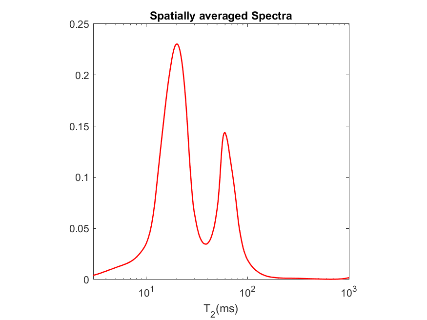
Example of 1D average spectrum |
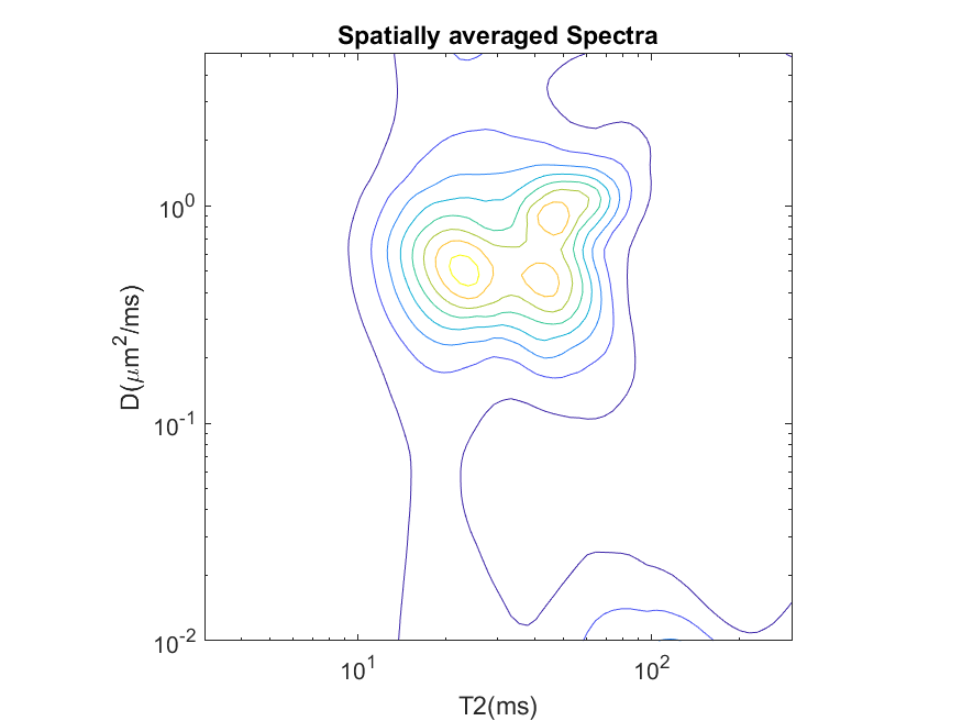
Example of 2D average spectrum |
When using optional arguments, the following syntax should be used:
plot_avg_spectra.sh -spect_imfile spect_imfile_name -outprefix outprefix_name -spatmaskfile spatmaskfile_name -ax_scale ax_scale_name -ax_lims ax_lims_values -color color_name -nlevel nlevel_value -linewidth linewidth_value -cbar tf -file_types file_types_name
plot_avg_spectra('spect_imfile','___','outprefix','___','spatmaskfile','___','ax_scale','___','ax_lims','___','nlevel','___','linewidth','___','cbar','___','file_types','___')
7.2.1. Required Inputs
spect_imfile:
The spectroscopic image to be visualized. The spectroscopic image must be in the
spectImagefileformat (e.g., as generated through DRSuite’s spectroscopic image estimation tool) as described here.spatmaskfile:
A binary spatial mask to use during visualization. This must be in the
spatmaskfileformat as described here, with the same spatial dimensions as the spectroscopic image, and will often be the same file that was used as input to the spectroscopic image estimation tool.outprefix:
A string specifying the filename prefix to use for the saved output image.
7.2.2. Optional Inputs
ax_scale:
A single string to control scaling of the axes denoting spectral sampling points. Accepts
'linear'or'log'only. If no input is provided, defaults to the spectral axes spacing fromaxes(i).spacingin spectroscopic image file.ax_lims:
Axis limits for the overlayed spectra. For 1D spectra use
[xmin xmax](defaults to the first and last samples fromaxes(1).sample). For 2D spectra use[ymin ymax xmin xmax](defaults fromaxes(1).sampleandaxes(2).sample). If length of this vector is other than 2 or 4 it shows an error.color:
Used to define Line color for 1D spectra or colormap for 2D spectra.
1D spectra: accepts a MATLAB color char/keyword (e.g.,
'r','red'). Recognized color keywords for 1D spectra:'r','g','b','c','m','y','k','w','red','green','blue','cyan','magenta','yellow','black','white'.2D spectra: Accepts a built-in colormap name (e.g.,
'jet'). Recognized colormaps for 2D spectra:'parula','jet','hsv','hot','cool','spring','summer','autumn','winter','gray','bone','copper','pink','lines','colorcube','prism','flag','white','turbo'.
nlevel:
Number of contour levels for 2D spectra plots (default: 12). Ignored for 1D spectra.
linewidth:
Line width for 1D line plots and 2D contour plots (default: 1.2).
file_types:
A string specifying the output image format (which will also be used as the filename suffix). Available options (not case sensitive):
fig,eps,pdf,bmp,jpg,png,tif,tiff. Defaults topngif not provided.
7.2.3. Output
An image file is saved using the specified filename prefix and output format.